SVM - Support Vector Machines
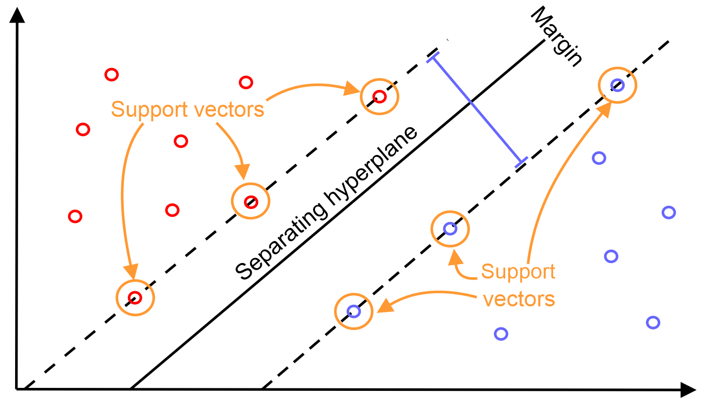
- The shortest distance between the observations and the threshold is called the margin. The distances between the observations and the threshold are the same and both reflect the margin. When the threshold is halfway between the two observations, the margin is as large as it can be
- observation: records on the tables/rows
- Maximal Margin Classifier: when we use the threshold that gives us the largest margin to make classifications
- Maximal Margin Classifiers are super sensitive to outliers in the training data and that makes them pretty lame
- Soft Margin: when we allow misclassifications, the distance between the observations and the threshold is called soft margin
- To make a threshold that is not so sensitive to outliers we must allow misclassifications
- choosing a threshold that allows a misclassifications is an example of the Bias/Variance Tradeoff.
- In other words, before we alloed misclassifications, we picked a threshold that was very sensitive to the training data (low bias) and it performed poorly when we got new data (high variance)
- In contrast, when we picked a threshold that was less sensitive to the training data and allowed misclassifications (higher bias) but it performed better when we got new data (low variance)
- How to determin which Soft Margin
- we use cross validation to determine how many classifications and observations to allow inside of the Soft Margin to get the best classification
- when we use a Soft Margin to determine the location of a threshold, then we are using a Soft Margin Classifier aka a Support Vector Classifier to classify observations
- the name Support Vector Classifier comes from the fact that the observations on the edge and within the Soft Margin are called Support Vectors
- when the data are 2-Dimentional, the Support Vector Classifier forms a line
- when the data are 3-Dimentional, the Support Vector Classifier forms a plane instead of a line, and we classify new observations by determining which side of the plane they are on.
- all flat affine subspaces are called hyperplanes
- Support Vector Classifier can
- handle outliers
- allow misclassifications
- handle overlapping classifications
- Support Vector Machines
- start with data in a relatively low dimension
- move the data into a higher dimension
- find a Support Vector Classifier that separates the higher dimensional data into two groups
- Question: How to transform data from low dimension to higher dimension?
- In order to make the mathematics possible, Support Vector Machines use something called Kernel Functions to systemaically find Support Vector Classifiers in higher dimensions

- Polynomial Kernel
- it systematically increases dimensions by setting d, the degree of the polynomial and the relationships between each pair of observations are used to find a Support Vector Classifier
- we can find a good value for d with Cross Validation
- Radial Kernel
- aka Radial Basis Function (RBF) Kernel
- it finds Support Vector Classifiers in infinite dimensions
- when using it on a new observation, the Radial Kernel behaves like a Weighted Nearest Neighbour model. The closest observations aka the nearest neighours have a lot of influence on how we classify the new observation and the observations that are further away have relatively little influence on the classification
- Polynomial Kernel
- Kernel Functions only calculate the relationships between every pair of points as if they are in the higher dimensions; they don’t actually do the transformation.
- This trick, calculating the high dimensional relationships without actually transforming the data to the higher dimensions, is called The Kernel Trick
- The Kernel Trick reduces the amount of computation required for Support Vector Machines by avoiding the math that transforms the data from low to high dimensions and it makes calculating relationships in the infinite dimensions used by the Radial Kernel possible
- In order to make the mathematics possible, Support Vector Machines use something called Kernel Functions to systemaically find Support Vector Classifiers in higher dimensions

The Polynomial Kernel
- Formula: (a*b+r)^d
- a and b refer to two different observations in the dataset
- r determines the coefficient of the polynomial
- d sets the degree of the polynomial
- r and d are determined using Cross Validation
- Dot Product
- the first terms multiplied together (x axis) + the second therms multiplied together (y axis) + the third terms multiplied together (z axis)
- the dot product gives us the high-dimensional coordinates for the data
- Polynomial Kernel computes relationships between pairs of observations
- once we deicde on values for r and d, we just plug in the observations and do the math to get the high-dimensional relationships
The Radial Kernel
aka the Radial Basis Function, RBF
- Formula:

- = high-dimensional relationships
- a and b refer to two different observations in the dataset
- the difference between the measurements is then squared, giving us the squared distance between the two observations
- the amount of influence one observation has on another is a function of the squared distance
- gamma, which is determined by Cross Validation, scales the squared distance, and thus, it scales the influence
- the further two observations are from each other, the less influence they have on each other
- Just like with the Polynomial Kernel, when we plug values into the Radial Kernel, we get the high-dimensional relationship
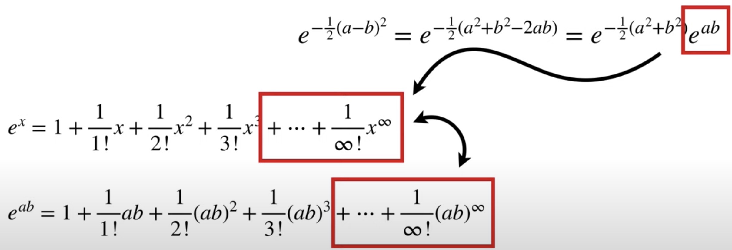
- Based on the Taylor Series Expansion, we can see when we plug numbers into the Radial Kernel and do the math. The value we get at the end is the relationship between the two points in infinite-dimensions
Taylor Series Expansion Based on The Radial Kernel
Taylor Series: f(x) can be split into an infinite sum
a can be any value as long as f(a) exists

set gamma as 1/2, and let’s create the Taylor Series Expansion of this last term

the derivative of e^x = e^x
set x0 = 0

when we added up a bunch of Polynomial Kernels with r=0 and d going from 0 to infinity, we got a Dot Product with coordinates for an infinite number of dimensions

Thus each term in this Taylor Series Expension contains a Polynomial Kernel with r=0 and d going from 0 to infinity
Dot Product for e^ab is

- we can verify that the Dot Product is correct by multiplying each term together
- add up the new terms to get the Taylor Series Expansion of e^ab

- we just multiply both parts of the Dot Product by the square root of this term

- we see that the Radial Kernel is equal to a Dot Product that has coordinates for an infinite number of dimensions

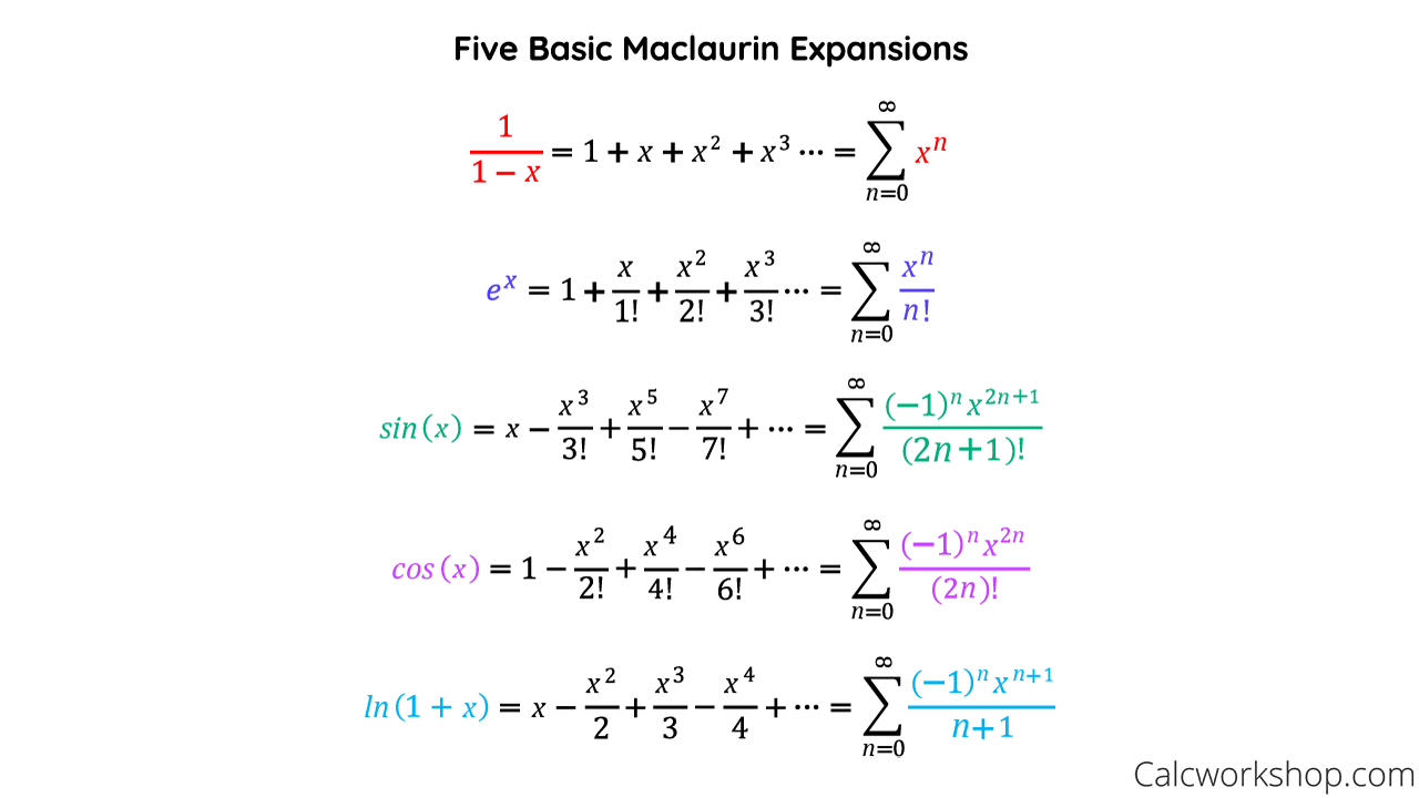
Maclaurine’s series
A Maclaurin Series is a Taylor Series where a = 0
